Logical functions in excel: and, or, xor and not

As demonstrated in the screenshot above, the formula works perfectly for all data types - numbers, dates and text values. When comparing text values, the formula checks them character-by-character in the alphabetic order. For example, it states that Apples in not between Apricot and Bananas because the second "p" in Apples comes before "r" in Apricot. Please see Using Excel comparison operators with text values for more details.

As you see, the IF /AND formula is simple, fast and almost universal. I say "almost" because it does not cover one scenario. The above formula implies that a value in column B is smaller than in column C, i.e. column B always contains the lower bound value and C - the upper bound value. This is the reason why the formula returns "No" for row 6, where A6 has 12, B6 - 15 and C6 - 3 as well as for row 8 where A8 is 24-Nov, B8 is 26-Dec and C8 is 21-Oct.

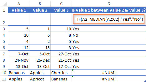
But what if you want your between formula to work correctly regardless of where the lower-bound and upper-bound values reside? In this case, use the Excel MEDIAN function that returns the median of the given numbers (i.e. the number in the middle of a set of numbers).

So, if you replace AND in the logical test of the IF function with MEDIAN, the formula will go like:

=IF(A2=MEDIAN(A2:C2),"Yes","No")

And you will get the following results:

As you see, the MEDIAN function works perfectly for numbers and dates, but returns the #NUM! error for text values. Alas, no one is perfect : )

If you want a perfect Between formula that works for text values as well as for numbers and dates, then you will have to construct a more complex logical text using the AND / OR functions, like this:

=IF(OR(AND(A2>B2, A2C2)), "Yes", "No")

Using the OR function in Excel

As well as AND, the Excel OR function is a basic logical function that is used to compare two values or statements. The difference is that the OR function returns TRUE if at least one if the arguments evaluates to TRUE, and returns FALSE if all arguments are FALSE. The OR function is available in all versions of Excel 2016 - 2000.

The syntax of the Excel OR function is very similar to AND:

OR(logical1, [logical2], …)

Where logical is something you want to test that can be either TRUE or FALSE. The first logical is required, additional conditions (up to 255 in modern Excel versions) are optional.

And now, let's write down a few formulas for you to get a feel how the OR function in Excel works.

Formula
Description

=OR(A2="Bananas", A2="Oranges")
Returns TRUE if A2 contains "Bananas" or "Oranges", FALSE otherwise.

=OR(B2>=40, C2>=20)
Returns TRUE if B2 is greater than or equal to 40 or C2 is greater than or equal to 20, FALSE otherwise.

=OR(B2=" ", C2="")
Returns TRUE if either B2 or C2 is blank or both, FALSE otherwise.

As well as Excel AND function, OR is widely used to expand the usefulness of other Excel functions that perform logical tests, e.g. the IF function. Here are just a couple of examples:

IF function with nested OR

=IF(OR(B2>30, C2>20), "Good", "Bad")

The formula returns "Good" if a number in cell B3 is greater than 30 or the number in C2 is greater than 20, "Bad" otherwise.

Excel AND / OR functions in one formula

Naturally, nothing prevents you from using both functions, AND & OR, in a single formula if your business logic requires this. There can be infinite variations of such formulas that boil down to the following basic patterns:

=AND(OR(Cond1, Cond2), Cond3)

=AND(OR(Cond1, Cond2), OR(Cond3, Cond4)

=OR(AND(Cond1, Cond2), Cond3)

=OR(AND(Cond1,Cond2), AND(Cond3,Cond4))

For example, if you wanted to know what consignments of bananas and oranges are sold out, i.e. "In stock" number (column B) is equal to the "Sold" number (column C), the following OR/AND formula could quickly show this to you:

=OR(AND(A2="bananas", B2=C2), AND(A2="oranges", B2=C2))

OR function in Excel conditional formatting

=OR($B2="", $C2="")

The rule with the above OR formula highlights rows that contain an empty cell either in column B or C, or in both.

For more information about conditional formatting formulas, please see the following articles:

Using the XOR function in Excel

In Excel 2013, Microsoft introduced the XOR function, which is a logical Exclusive OR function. This term is definitely familiar to those of you who have some knowledge of any programming language or computer science in general. For those who don't, the concept of 'Exclusive Or' may be a bit difficult to grasp at first, but hopefully the below explanation illustrated with formula examples will help.

The syntax of the XOR function is identical to OR's :

XOR(logical1, [logical2],…)

The first logical statement (Logical 1) is required, additional logical values are optional. You can test up to 254 conditions in one formula, and these can be logical values, arrays, or references that evaluate to either TRUE or FALSE.

In the simplest version, an XOR formula contains just 2 logical statements and returns:

• TRUE if either argument evaluates to TRUE.
• FALSE if both arguments are TRUE or neither is TRUE.

This might be easier to understand from the formula examples:

Formula
Result
Description

=XOR(1>0, 2<1)
TRUE
Returns TRUE because the 1st argument is TRUE and the 2nd argument is FALSE.

=XOR(1<0, 2<1)
FALSE
Returns FALSE because both arguments are FALSE.

=XOR(1>0, 2>1)
FALSE
Returns FALSE because both arguments are TRUE.

When more logical statements are added, the XOR function in Excel results in:

• TRUE if an odd number of the arguments evaluate to TRUE;
• FALSE if is the total number of TRUE statements is even, or if all statements are FALSE.

The screenshot below illustrates the point:

If you are not sure how the Excel XOR function can be applied to a real-life scenario, consider the following example. Suppose you have a table of contestants and their results for the first 2 games. You want to know which of the payers shall play the 3rd game based on the following conditions:

• Contestants who won Game 1 and Game 2 advance to the next round automatically and don't have to play Game 3.
• Contestants who lost both first games are knocked out and don't play Game 3 either.
• Contestants who won either Game 1 or Game 2 shall play Game 3 to determine who goes into the next round and who doesn't.

A simple XOR formula works exactly as we want:

=XOR(B2="Won", C2="Won")

And if you nest this XOR function into the logical test of the IF formula, you will get even more sensible results:

=IF(XOR(B2="Won", C2="Won"), "Yes", "No")

Using the NOT function in Excel

The NOT function is one of the simplest Excel functions in terms of syntax:

NOT(logical)

You use the NOT function in Excel to reverse a value of its argument. In other words, if logical evaluates to FALSE, the NOT function returns TRUE and vice versa. For example, both of the below formulas return FALSE:

=NOT(TRUE)

=NOT(2*2=4)

Why would one want to get such ridiculous results? In some cases, you might be more interested to know when a certain condition isn't met than when it is. For example, when reviewing a list of attire, you may want to exclude some color that does not suit you. I'm not particularly fond of black, so I go ahead with this formula:

=NOT(C2="black")

As usual, in Microsoft Excel there is more than one way to do something, and you can achieve the same result by using the Not equal to operator: =C2<>"black".

If you want to test several conditions in a single formula, you can use NOT in conjunctions with the AND or OR function. For example, if you wanted to exclude black and white colors, the formula would go like:

=NOT(OR(C2="black", C2="white"))

And if you'd rather not have a black coat, while a black jacket or a back fur coat may be considered, you should use NOT in combination with the Excel AND function:

=NOT(AND(C2="black", B2="coat"))

Another common use of the NOT function in Excel is to reverse the behavior of some other function. For instance, you can combine NOT and ISBLANK functions to create the ISNOTBLANK formula that Microsoft Excel lacks.

As you know, the formula =ISBLANK(A2) returns TRUE of if the cell A2 is blank. The NOT function can reverse this result to FALSE: =NOT(ISBLANK(A2))

And then, you can take a step further and create a nested IF statement with the NOT / ISBLANK functions for a real-life task:

=IF(NOT(ISBLANK(C2)), C2*0.15, "No bonus :(")

Translated into plain English, the formula tells Excel to do the following. If the cell C2 is not empty, multiply the number in C2 by 0.15, which gives the 15% bonus to each salesman who has made any extra sales. If C2 is blank, the text "No bonus :(" appears.

In essence, this is how you use the logical functions in Excel. Of course, these examples have only scratched the surface of AND, OR, XOR and NOT capabilities. Knowing the basics, you can now extend your knowledge by tackling your real tasks and writing smart elaborate formulas for your worksheets.

You may also be interested in